NBLASTing FlyWire neurons against Janelia hemibrain
Let’s say you have traced a couple neurons in FlyWire and want to find the same neurons in the Janelia hemibrain dataset. If you’re lucky we’ve been able to identify the cell type for you (see the annotations tutorial). If not, you could try manually hunting for your neurons of interests but that’s rather tedious. Better to use NBLAST to find potential matches for you!
To run below code you will need these libraries:
fafbsegnavis (version >= 0.5.2)
flybrains (version >=0.1.4) including the optional Saalfeld transforms (see docs on how to download them)
Let’s jump right in!
>>> import navis
>>> import flybrains

>>> from fafbseg import flywire
navis wraps neuprint-python and adds convenience functions which
we will use later on to visualize potential matches.
A quick outline of what we will do now:
Load a couple FlyWire neurons
Turn the neurons into dotprops for NBLASTing
Transform the dotprops to the
JRC2018Ftemplate spaceMirror left-hand-side FlyWire dotprops to the right
Prune the FlyWire dotprops to the approximate hemibrain volume
NBLAST against ~26k hemibrain neurons
Inspect potential matches
OK, first to get some FlyWire neurons. For demonstration purposes, I will use some olfactory projection neurons from the left and the right since we know the ground truth for those:
>>> # Use the public release data for FlyWire
>>> flywire.set_default_dataset("public")
Default dataset set to "public"
>>> # Root IDs of three PNs
>>> root_ids = [720575940613852614, 720575940626542891, 720575940621770759]

>>> # Fetch L2 dotprops for those neurons
>>> fw_dps = flywire.get_l2_dotprops(root_ids)
>>> # A quick visualization
>>> # Note we're plotting the FLYWIRE brain on top of it
>>> fig, ax = navis.plot2d(
...     [fw_dps, flybrains.FLYWIRE], dps_scale_vec=1000, lw=1.5, figsize=(12, 12)
... )
>>> ax.azim = ax.elev = -90
>>> ax.set_box_aspect(None, zoom=1)
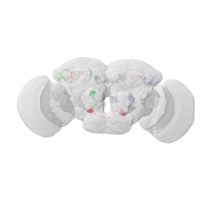
the green PN should be entirely contained in the hemibrain volume
the red bilateral PN will be truncated but we should still be able to find a match
the blue PN on the right we will need to mirror to the left
Next: transform the dotprops to JRC2018F brain space. This template brain is an average of several brains and as such is symmetric which means we can mirror things really easily. It is also in microns! Both the template brain as well as the transforms to/from it are provided by the Saalfeld lab (Janelia), in particular John Bogovic.
>>> fw_dps_2018f = navis.xform_brain(fw_dps, source="FLYWIRE", target="JRC2018F")
INFO : Pre-caching deformation field(s) for transforms... (navis)
Transform path: FLYWIRE -> JRCFIB2022M -> FAFB14 -> FAFB14um -> JRC2018F
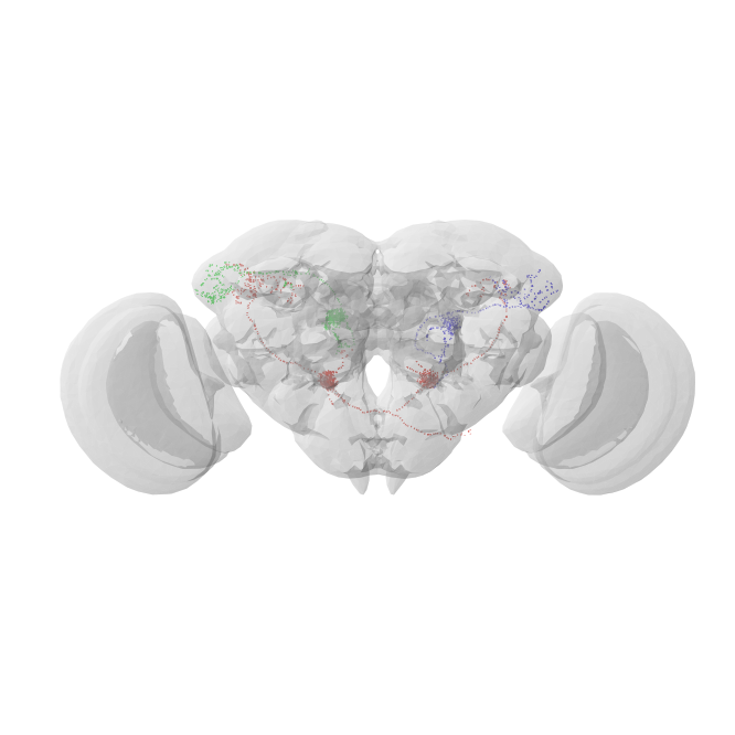
For a quick sanity check let’s plot our transformed FlyWire dotprops on top of the JRC2018F brain mesh:
>>> fig, ax = navis.plot2d(
...     [fw_dps_2018f, flybrains.JRC2018F], dps_scale_vec=1, lw=1.5, figsize=(12, 12)
... )
>>> ax.azim = ax.elev = -90
>>> ax.set_box_aspect(None, zoom=1)
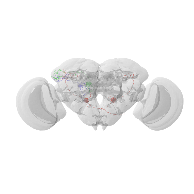
Now mirror 720575940621770759 to the other side of the brain:
>>> mirrored = navis.mirror_brain(fw_dps_2018f.idx[720575940621770759], template="JRC2018F")

>>> # Combine unmirrored and mirrored neurons
>>> fw_dps_2018f_right = (
...     fw_dps_2018f.idx[[720575940613852614, 720575940626542891]] + mirrored
... )
A final sanity check:
>>> fig, ax = navis.plot2d(
...     [fw_dps_2018f_right, flybrains.JRC2018F], dps_scale_vec=1, lw=1.5, figsize=(12, 12)
... )
>>> ax.azim = ax.elev = -90
>>> ax.set_box_aspect(None, zoom=1)
Now prune the neurons to the approximate bounding box of the hemibrain.
>>> bbox = flybrains.JRCFIB2018Fraw.bbox

>>> # Here we transform the bounding box from hemibrain into JRC2018F space
>>> # You can ignore the warning about too many points being outside the volume
>>> bbox_2018f = navis.xform_brain(bbox, source="JRCFIB2018Fraw", target="JRC2018F")
Transform path: JRCFIB2018Fraw -> JRCFIB2018F -> JRCFIB2018Fum -> JRC2018F
WARNING : A suspiciously large fraction (44.4%) of 54 points appear to be outside the H5 deformation field. Please make doubly sure that the input coordinates are in the correct space/units (navis)
Subset the neurons to the bounding box:
>>> fw_dps_2018f_final = navis.in_volume(fw_dps_2018f_right, bbox_2018f)
The final final sanity check:
>>> fig, ax = navis.plot2d(
...     [fw_dps_2018f_final, bbox_2018f, flybrains.JRC2018F],
...     dps_scale_vec=1,
...     lw=1.5,
...     figsize=(10, 12),
... )
>>> ax.azim = ax.elev = -90
>>> ax.set_box_aspect(None, zoom=1)
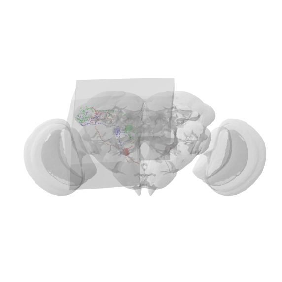
OK that looks good! For what it’s worth: we’re doing these visualization only for illustrative purposes but I do recommend you spot-check your data as you process it.
Next we need to get dotprops for all hemibrain neurons. If you want to do this yourself you would need to:
Download a hemibrain skeleton dump or individual skeletons from neuprint
Generate dotprops from the skeletons (don’t forget to resample to 1 micron!)
Transform to JRC2018U template space
Lucky for you, I already did that and you can download the pickled data from my Google drive:
https://drive.google.com/file/d/1pcPpiDdG_VxnY74ttXVOLDbhDlkIq3Ad/view?usp=sharing (~1.3Gb)
First we need to load that file:
>>> import pickle

>>> with open("hemibrain_dotprops_jrc2018f.pkl", "rb") as f:
>>>     hemi_dps_2018f = pickle.load(f)

>>> print(f"We have dotprops for {len(hemi_dps_2018f)} hemibrain neurons")
We have dotprops for 25607 hemibrain neurons
Now we are all set for starting the NBLAST. Here, we will be using
navis.nblast_smart. This function works by first running a
pre-NBLAST on highly simplified dotprops and then running a full NBLAST
only for interesting (i.e. high-scoring) pairs of neurons.
This is much faster and perfectly sufficient if you are only trying to
find some decent matches. For quantitative analyses you should go for a
full NBLAST with navis.nblast though!
>>> scores = navis.nblast_smart(
...    fw_dps_2018f_final,
...    hemi_dps_2018f,
...    scores="mean",
...    criterion="N",
...    t=10,
...    normalized=True,
... )
- For reference:
scores are normalized such that 1 is a perfect match
we get the ‘mean’ of the forward and reverse scores
the full NBLAST will be run on the top 10 target of the pre-NBLAST for each FlyWire neuron
Inspect the scores:
>>> scores
| 730562993 | 1038079690 | 706948318 | 297938585 | 5813063224 | 1751943911 | 1624418395 | 1686190133 | 5812997194 | 5813021017 | ... | 1817799390 | 1793014384 | 575768294 | 324790113 | 2069647778 | 387507495 | 328713871 | 1473695252 | 1042651606 | 390245740 | |
|---|---|---|---|---|---|---|---|---|---|---|---|---|---|---|---|---|---|---|---|---|---|
| 720575940613852614 | -0.317906 | -0.824387 | -0.689619 | -0.646354 | -0.570998 | -0.713661 | -0.822287 | -0.770065 | -0.880665 | -0.494713 | ... | -0.826107 | -0.685051 | -0.502179 | -0.583609 | 0.255378 | -0.384741 | -0.881489 | -0.739343 | -0.050083 | -0.479143 |
| 720575940626542891 | -0.338047 | -0.819632 | -0.644048 | -0.599290 | -0.418029 | -0.880746 | -0.880055 | -0.847185 | -0.880046 | -0.332676 | ... | -0.880994 | -0.321261 | -0.525081 | -0.546979 | -0.542610 | -0.330692 | -0.845514 | -0.751669 | -0.546660 | -0.300891 |
| 720575940621770759 | -0.284522 | -0.863342 | -0.641244 | -0.851290 | -0.732890 | -0.881525 | -0.850988 | -0.780079 | -0.881242 | -0.470615 | ... | -0.882160 | -0.340289 | -0.456179 | -0.809773 | -0.214426 | -0.630141 | -0.880620 | -0.643453 | -0.394046 | -0.445954 |
3 rows × 25607 columns
The index/columns are the FlyWire root and hemibrain body IDs, respectively
Next we will get the, say, top 3 matches for each of our query neurons:
>>> import numpy as np
>>> import pandas as pd


>>> def get_top(N=3):
...     """Produce matrix with top N matches."""
...     # For each row get the order of columns in ascending score
...     ix_srt = np.argsort(scores.values, axis=1)[:, ::-1]
...
...     # Populate a DataFrame
...     df = pd.DataFrame([])
...
...     for i in range(N):
...         df[f"top_{i+1}"] = scores.columns[ix_srt[:, i]]
...         df[f"top_{i+1}_score"] = scores.values[np.arange(scores.shape[0]), ix_srt[:, i]]
...
...     df.index = scores.index
...
...     return df


>>> top_3 = get_top(N=3)
>>> top_3
| top_1 | top_1_score | top_2 | top_2_score | top_3 | top_3_score | |
|---|---|---|---|---|---|---|
| 720575940613852614 | 2064165421 | 0.726949 | 666818300 | 0.435697 | 5813103893 | 0.391695 |
| 720575940626542891 | 693483018 | 0.631542 | 635062078 | 0.375847 | 5813056596 | 0.368527 |
| 720575940621770759 | 733316908 | 0.675452 | 886812643 | 0.518861 | 754538881 | 0.395918 |
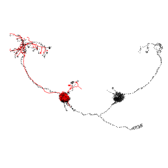
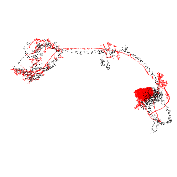
It looks like we have reasonably good hits for all three PNs. Let’s check those out - black is the hemibrain neuron, red is the top hit:
>>> fig, ax = navis.plot2d(
...     [fw_dps_2018f_right.idx[720575940613852614], hemi_dps_2018f.idx[2064165421]],
...     figsize=(12, 12),
...     method="3d_complex",
...     lw=1.5,
...     c=["k", "r"],
... )
>>> ax.azim = ax.elev = -90
>>> ax.set_box_aspect(None, zoom=1)
>>> fig, ax = navis.plot2d(
...     [fw_dps_2018f_right.idx[720575940626542891], hemi_dps_2018f.idx[693483018]],
...     figsize=(12, 12),
...     method="3d_complex",
...     lw=1.5,
...     c=["k", "r"],
... )
>>> ax.azim = ax.elev = -90
>>> ax.set_box_aspect(None, zoom=1)
>>> fig, ax = navis.plot2d(
...     [fw_dps_2018f_right.idx[720575940621770759], hemi_dps_2018f.idx[733316908]],
...     figsize=(12, 12),
...     method="3d_complex",
...     lw=1.5,
...     c=["k", "r"],
... )
>>> ax.azim = ax.elev = -90
>>> ax.set_box_aspect(None, zoom=1)
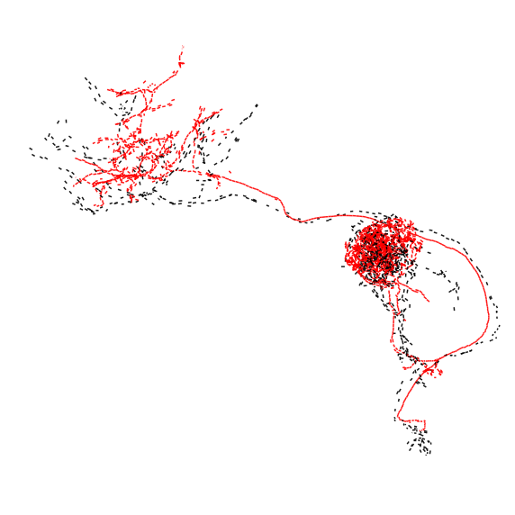
Based on the dotprops, all matches look decent. Moving forward, you could load the skeletons or meshes from neuprint (see this tutorial), transform them to a common space with the FlyWire neurons and co-visualize them.