Fetching neurons

In this tutorial you will learn to fetch various representations (meshes, skeletons and dotprops) for FlyWire neurons.

First up: imports!

>>> import navis
>>> from fafbseg import flywire

We will run our tutorial using the public dataset. To make our life easier we will set the default dataset:

>>> flywire.set_default_dataset("public")

Default dataset set to "public"

OK, with that out of the way let’s load some neurons:

>>> n = flywire.get_mesh_neuron(720575940625431866)
>>> n

type	navis.MeshNeuron
name	None
id	720575940625431866
units	1 nanometer
n_vertices	309801
n_faces	622597

Now we can use navis to plot the neuron:

>>> fig, ax = navis.plot2d(n, color="red")
>>> ax.azim = ax.elev = -90

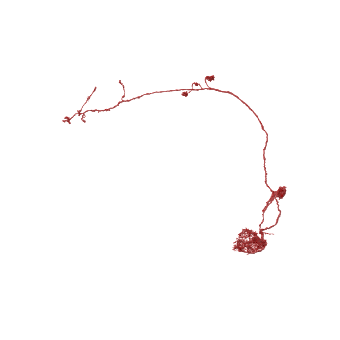
Note that FlyWire neurons are very detailed: the above neuron has over half a million faces! That makes working with them slow and it’s a good idea to downsample them if possible. You can use navis.downsample_neuron to reduce the number of faces in a neuron

Alternatively, you can use skeleton representations of the neurons which are much faster to work with and can be used to compute various statistics such as the total length of the neuron.

For the public snapshots (630 and 783) we provide precomputed, high quality skeletons for all proofread(!) neurons via get_skeletons():

>>> sk = flywire.get_skeletons(720575940625431866)
>>> sk

type	navis.TreeNeuron
name	skeleton
id	720575940625431866
n_nodes	3885
n_connectors	None
n_branches	764
n_leafs	859
cable_length	2236532.0
soma	[467, 470, 472, 475, 477, 479, 480, 631, 635, ...
units	1 nanometer

These skeletons are also available for bulk download via this Github repository: https://github.com/flyconnectome/flywire_annotations

What if there is no precomputed skeleton available for your neuron(s) of interest?

In that case you have two options to generate skeletons yourself: 1. Generate a high-res skeleton from scratch (slow) 2. Generate a low-res skeleton using the L2 cache (fast)

Let’s first demo the high-res skeleton:

%%time

>>> # Generate a high-res skeleton from scratch
>>> sk = flywire.skeletonize_neuron(720575940625431866, progress=False)
>>> sk

CPU times: user 20.2 s, sys: 2.12 s, total: 22.3 s
Wall time: 27.4 s

type	navis.TreeNeuron
name	None
id	720575940625431866
n_nodes	10326
n_connectors	None
n_branches	740
n_leafs	854
cable_length	2491188.964376
soma	12908
units	1 nanometer

As you can see skeletonization is an expensive process and it can take several minutes on large neurons. Our examples neuron took around 30s on a laptop which is about average.

If you need to skeletonize many neurons you can use fafbsegb.flywire.skeletonize_neurons_parallel() to speed things up.

Also note that the default settings for the skeletonization work well enough for 9 out of 10 neurons but you might have to play around with them if the skeleton looks odd or takes very long to generate.

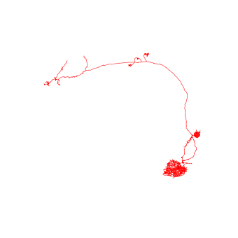
>>> fig, ax = navis.plot2d(sk, color="red")
>>> ax.azim = ax.elev = -90

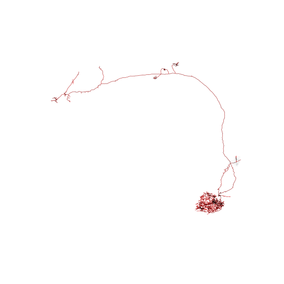
For comparison, lets plot mesh (transparent grey) and skeleton (red) side-by-side:

>>> fig, ax = navis.plot2d([sk, n], color=["r", (.3, .3, .3, 0.1)], figsize=(10, 10), method='3d_complex')
>>> ax.azim = ax.elev = -90

We can also use plot3d instead of plot2d. Try zooming in to see how the skeleton compares to the mesh.

>>> navis.plot3d([sk, n], color=["r", (0.3, 0.3, 0.3, 0.3)])

If you don’t need high-res meshes or skeletons, you might want to take a look at on-the-fly L2 skeletons. These are coarser but much faster to generate:

>>> # Time how long it takes to grab an L2 skeleton
>>> %time l2_sk = flywire.get_l2_skeleton(720575940625431866)

CPU times: user 135 ms, sys: 9.33 ms, total: 144 ms
Wall time: 3.1 s

Note

For NBLASTs, there is also a function for on-the-fly dotprops:

>>> l2_dp = flywire.get_l2_dotprops(720575940625431866)

Let’s compare the full-res and L2 skeleton:

>>> fig, ax = navis.plot2d([sk, l2_sk], color=["r", "c"], method='3d_complex')
>>> ax.azim = ax.elev = -90

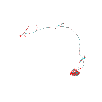
These L2 skeletons (or dotprops) are good enough for most morphological analyses and NBLAST!

Note

Have a look at the tutorials for navis to learn more about what you can do with the neurons.